Localizations Features
Self-Localization of the robots relies mainly on features detected through image recognition. That includes the field lines, the center circle and the penalty marks. The detection modules of all three use a shared pre-processing step. It provides a grid of scan lines divided into regions that show the field, something white, or something else. There, the image processing flow splits into modules for detecting the specific features. Then the detected lines, center circle and penalty mark are also merged again into composite localization features, such as line intersections, center circle with center line and penalty mark with penalty area.
Scan Grid / Scan Line Regions
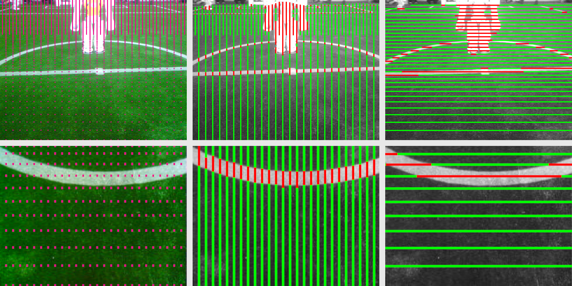
As a pre-processing step we scan in image in horizontal and vertical lines, that are close enough together to find field lines, penalty marks and the ball. Therefore, we compute the ScanGrid dynamically depending on the vertical orientation of the camera. The distance between to grid points roughly corresponds to a distance of a bit less than the expected width of a field line at that position in the image. The resulting grid can be seen in the left half of the following image.
Then, the scans are executed by the ScanLineRegionizer module, which provides the vertical and horizontal scan line regions shown in the middle and on the right side. It divides the scan lines into regions and classifies them as either field, white or a generic class none that stands for everything else. Regions classified as white are shown in red for better visibility.
The scan line regions are generated without prior color calibration. In order to obtain reliable results even under dynamic lighting conditions, the color ranges initially assigned to the various color classes are recalculated for each image. For the determination of the beginning and end of the regions, no fixed color ranges are used at all but only local comparison points. The steps in detail are as follows:
- Define the scan lines
- Limit the range of the scan lines to exclude parts outside the field boundary and where the robot sees itself.
- Detect edges and create temporary regions in between
- Compare luminance between neighboring grid points. If the difference is above a threshold, find the position with the highest luminance change in between.
- Assign a YHS triple to each region, that represents its color.
- Classify field regions
- Unite all neighboring regions of similar colors that are in the possible field color range in union-find-trees.
- Classify all union-regions that span enough pixels as field and determine the field color range.
- Classify the remaining regions that match the field color range as field.
- Classify white regions
- All regions significantly brighter than both neighboring regions.
- Infer white color range from field color range and approximated image average luminance and saturation.
- All regions that were not previously labeled as field and match the white color range.
- Fill small gaps between field and white regions
- Sometimes small regions that lie between field and white cannot be classified with certainty. They become split in the middle.
- Merge neighboring regions of the same class
The horizontal and vertical scan lines are currently calculated independently and don't become synchronized. Therefore, a grid point classified as one class in the horizontal scan lines might be classified differently in the vertical scan lines.
Field Line Detection
Line Spots
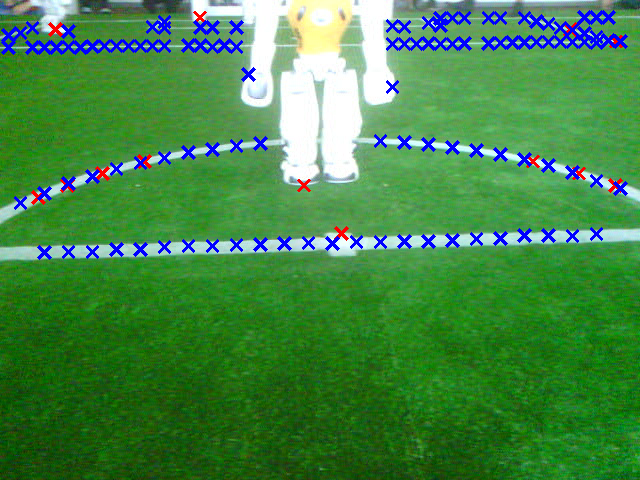
The perception of field lines and the center circle by the LinePerceptor rely on the scanline regions. In order to find horizontal lines in the image, adjacent white vertical regions that are not within a perceived obstacle are combined to line segments (shown in blue). Correspondingly, vertical line segments are constructed from white horizontal regions (shown in red). These line segments and the center points of their regions, called line spots, are then projected onto the field.
Detecting Lines
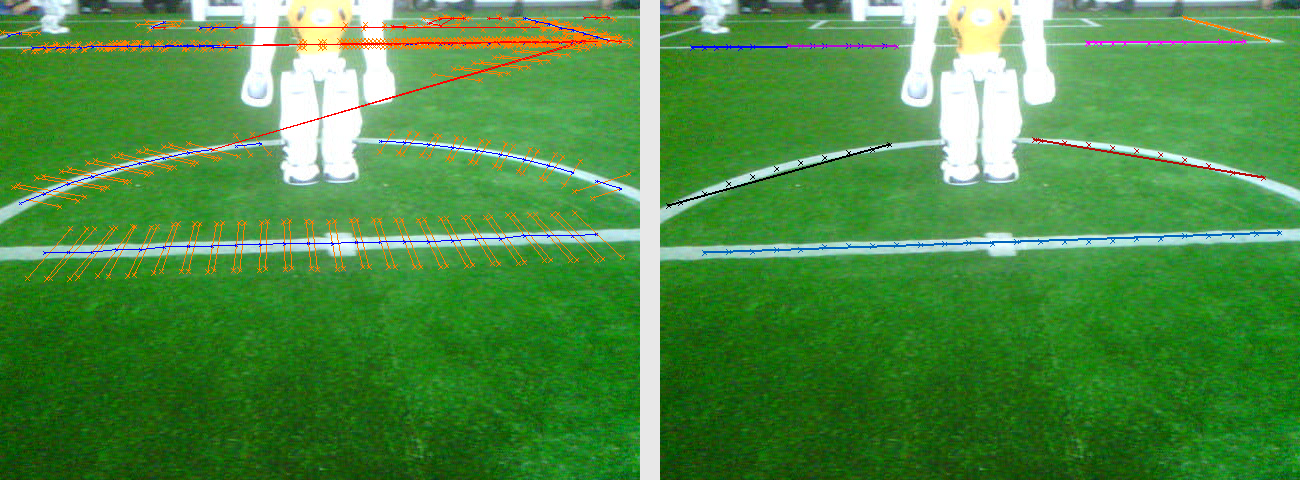
Using linear regression of the line spots, they are then merged together and extended to larger line segments. During this step, line segments are only merged together if they pass a white test. For this we sample points close but definitely outside the presumed line in a regular interval to both sides of the checked line segments. A given ratio of the checked points need to be less bright and more saturated than their corresponding point on the presumed line segment. Only then the line spots are merged to a segment, otherwise the presumed segment get rejected. The left image shows this process, with accepted line segments in blue, rejected segments in red and the checked points in orange. The right image shows the eventually found line percepts.
Detecting the Center Circle
Besides providing the LinesPercept containing perceived field lines, the LinePerceptor also detects the center circle in an image if it is present. In order to do so, when combining line spots to line segments, their field coordinates are also fitted to circle candidates. After the LinesPercept was computed, spots on the circle candidates are then projected back into the image and adjusted so they lie in the middle of white regions in the image. These adjusted spots are then again projected onto the field and it is once again tried to fit a circle through them, excluding outliers.
If searching for the center circle using this approach did not yield any results, another method of finding the center circle is applied. We take all previously detected lines whose spots describe an arc and accumulate the center points of said arcs to cluster them together. If one of these clusters contains a sufficient number of center points, the average of them is considered to be the center of the center circle.
If a potential center circle was found by any of these two methods, it is accepted as a valid center circle only if – after projecting spots on the circle back into the image – at least a certain ratio of the corresponding pixels is white, using the same whiteness test as in the line detection.
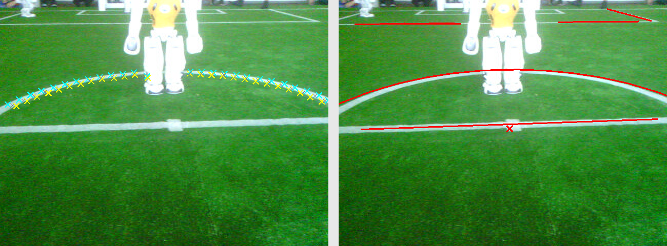
The image shows the detected inner and outer edge of the circle used for finding the circle center point. The right side shows the filtered line and circle percepts in the FieldLines representation.
Line Intersections
Part of the self-localization is the usage of line intersections as landmarks. Not only is the position of an intersection important but also the type of intersection. Previously, we determined the location and type of the intersections by calculating where perceived field lines coincide. This method proved to be very reliable regarding the detection of intersections. The classification however only provides reliable results for intersections that are not beyond 3 m. Because of this, we implemented a convolutional neural network that classifies all intersections that are further than 3 m away. Intersections closer than 3 m are still handled by the hand-crafted algorithm.
Both classification approaches work on candidates, i.e. two lines that possibly intersect. To generate candidates, each previously detected line will be compared to all other detected lines, excluding those that are known to be part of the center circle. Because of the way the field is set up an intersection is only possible if the inclination of two compared lines in field coordinates is roughly 90°.
We divide the intersections into three types, which we call L, T, and X, corresponding to the shape formed by the lines on the field. The IntersectionsPercept representation then stores the type of each intersection as well as its position, its basis lines, and its rotation.
Geometric approach
For each candidate the point of intersection of the two lines is calculated. In order to be valid, this point must lie in between both detected line segments. The classification of intersection types uses the endpoints of the involved lines. This means that intersections lying clearly in-between both lines are of type X while those that are clearly inside one line but roughly at one end of the other are considered to be of type T. If the point of intersection lies roughly at the ends of both lines, it is assumed to belong to an L-type intersection.
In case that parts of both lines are seen but the point of intersection does not lie on either line - e.g. because an obstacle is standing in front of the intersection point – the lines will be virtually stretched to some extent so that the point of intersection lies roughly at their ends. The possible distance by which a line can be extended depends on the length of its recognized part.
CNN approach
For the CNN a candidate consists of a 32 × 32 pixels grayscale image of the intersection which will be input into the neural network where it will be classified. The network has four output classes: L, T, X and NONE. The first three classes represent the three different intersection types on the field. A candidate will be classified as NONE, if no intersection can be seen on the image.
Close to 8000 images were used to train the model. These images were extracted from logs of B-Human games from 2019 and 2021 under different lighting conditions.
Penalty Mark Perception
The penalty mark is one of the most prominent features on the field since it only exists twice. In addition, it is located in front of the penalty area and can thereby be easily seen by the goal keeper. By eliminating false positive detections, the penalty mark can be used as a reliable feature for self-localization. This is achieved by limiting the detection distance to 3 m and by using a convolutional neural network for classification of candidates.
Approach
Similar to the ball detection, the image is first searched for a number of candidates which are checked afterward for being the actual penalty mark. The search for candidates and the actual check are separated into different modules. This allows us to handle the generation of candidate regions differently depending on the camera, while the verification is the same in both cases.
Finding Candidate Regions
Upper Camera
For images from the upper camera the PenaltyMarkRegionsProvider generates the penalty mark candidates. First, it collects all regions of the scanned low resolution grid that were not classified as green, i.e. white, black, and unclassified regions. In addition, the regions are limited to a distance of 3 m from the robot, assuming they represent features on the field plane. Vertically neighboring regions are merged and the amount of pixels that were actually classified as white in each merged region is collected. Regions at the lower end and the upper end of the scanned area are marked as invalid, i.e. there should be a field colored region below and above each valid region. The regions are horizontally grouped using the Union Find approach. To achieve a better connectedness of, e.g., diagonal lines, each region is virtually extended by the expected height of three field line widths when checking for the neighborhood between regions. For each group, the bounding box and the ratio between white and non-green pixels is determined. For all groups with a size similar to the expected size of a penalty mark that are sufficiently white and that do not contain invalid regions, a search area for the center of the penalty mark and a search area for the outline of the penalty mark are computed. As the search will take place on 16 × 16 cells, the dimensions are extended to multiples of 16 pixels.
Lower Camera
For lower camera images we use a CNN on the full image for candidate generation. Running the network on the full image in real time is possible only because we use the lower camera at lower resolution, so this not a viable approach for the upper camera. The network acts as a multi-perceptor, detecting balls, robots and penalty marks at the same time. Only the penalty mark prediction with the highest confidence becomes a candidate to be double-checked.
Checking Penalty Mark Candidates
We use a single CNN for the binary classification of the candidates belonging either to class “Spot” or “No Spot”. Running the network is handled in the PenaltyMarkPerceptor module. The network’s architecture is described in the following table:
| Layer Type | Output Size | Number of Parameters |
|---|---|---|
| Input | 32 × 32 × 1 | |
| Convolutional | 30 × 30 × 8 | 80 |
| Batch Normalization | 30 × 30 × 8 | 32 |
| Convolutional | 28 × 28 × 16 | 1168 |
| Max Pooling | 14 × 14 × 16 | 0 |
| Batch Normalization | 14 × 14 × 16 | 64 |
| Convolutional | 12 × 12 × 8 | 1160 |
| Max Pooling | 6 × 6 × 8 | 0 |
| Flatten | 288 | 0 |
| Dense | 64 | 18496 |
| Dense | 2 | 130 |
The network was trained on over 40000 images obtained from logs of B-Human games between 2019 and 2021 with various lighting conditions and different applications of lines on the field. The center of the spot is assumed to be the center of the provided region which is not always completely accurate but close enough in most cases. In the special case of a penalty shootout, we assume the position of the ball to also be the position of the penalty spot, since the ball must be located on the penalty spot, blocking the view of the mark itself.