SimRobot¶

The B-Human software package uses the physical robotics simulator SimRobot¹² as front end for software development. The simulator is not only used for working with simulated robots, but it also functions as graphical user interface for replaying log files and connecting to physical robots via Ethernet or Wi-Fi.

Architecture¶

Four dynamic libraries are created when SimRobot is built. These are SimulatedNao, SimRobotCore2, SimRobotCore2D and SimRobotEditor³.

SimRobotCore2 is the simulation core. It is the most important part of the SimRobot application, because it models the robots and the environment, simulates sensor readings, and executes commands given by the controller or the user. The core is platform-independent and it is connected to a user interface and a controller via a well-defined interface.

SimRobotCore2D is a simulation core for 2D simulations. It has the same role as SimRobotCore2 and is selected based on the suffix of the loaded scene filename (.ros2d instead of .ros2).

SimRobotCommon is a static library which contains code shared by SimRobotCore2 and SimRobotCore2D.

The library SimulatedNao is in fact the controller that consists of the two projects SimulatedNao and Controller. SimulatedNao creates the code for the simulated robot. This code is linked together with the code created by the Controller project to the SimulatedNao library. In the scene files, this library is referenced by the controller attribute within the Scene element.

The following graph shows the most important parts of SimRobot (excluding third-party libraries). Rectangles represent projects that create the corresponding library or executable. Dynamic libraries are represented as rectangles with rounded sides. Static libraries are depicted as rectangles with rounded corners. Solid arrows mean "creates". Dotted ones mean "used by".

B-Human Toolbar¶

The B-Human toolbar is part of the general SimRobot toolbar which can be found at the top of the application window. It allows setting the representations MotionRequest and HeadAngleRequest to frequently used values.

Button	Function
	Lets the robot stand up.
	Lets the robot sit down.
	Allows moving the robot's head by hand.

Scene View¶

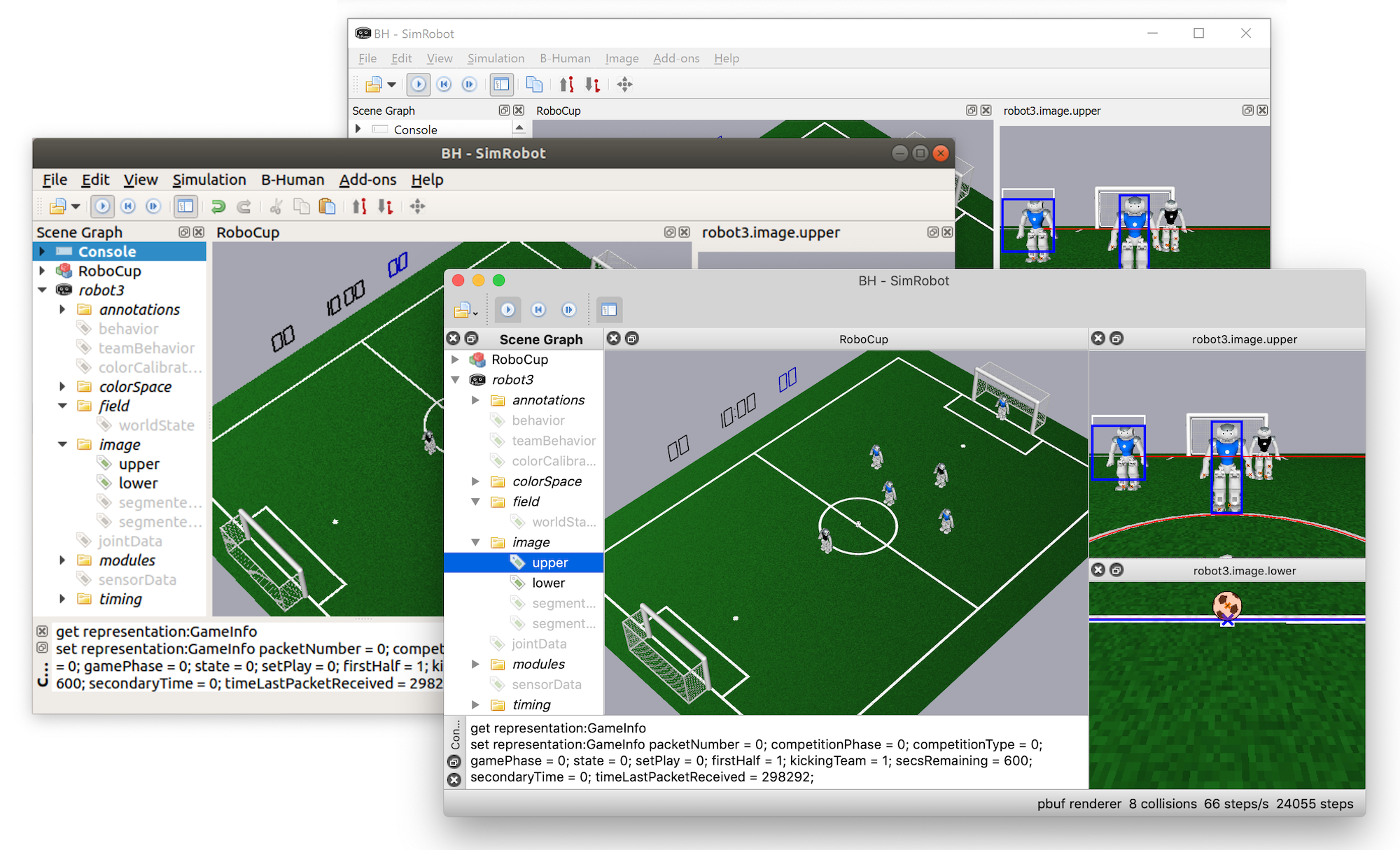
The scene view (e.g. the central view in the image below) appears if the scene is opened from the scene graph, e.g. by double-clicking on the entry RoboCup. The view can be translated by dragging, rotated by dragging with the Shift key pressed, zoomed, and it supports several mouse operations on objects:

• Left-clicking an object allows dragging it to another position. Robots and the ball can be moved in that way.
• Left-clicking while pressing the Shift key allows rotating objects around their centers. The axes of the rotating objects can be selected first by pressing the x, y or z key, before pressing and holding the Shift key.
• Double-clicking an active robot selects it. Robots are active if they are defined in the compound robots in the scene description file (cf. this section). Robot console commands are sent to the selected robot only (see also the command robot).

The following image shows SimRobot running on Windows, Linux, and macOS. The left pane shows the scene graph, the center pane shows a scene view, and on the right there are two views showing the images of both cameras. The console window is shown at the bottom.

Information Views¶

In the simulator, information views are used to display debugging output such as debug drawings. Such output is generated by the robot control program, and it is sent to the simulator via message queues (this section). The views are interactively created using the console window, or they are defined in a script file. Since SimRobot is able to simulate more than a single robot, the views are instantiated separately for each robot. There are 13 kinds of information views, which are structured here into the five categories perception, cognition, motion, and others. All information views can be selected from the scene graph (cf. the left widget in the previous image).

Perception¶

Image Views¶

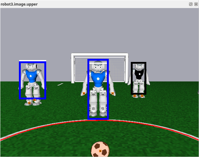
An image view displays debug information in the coordinate system of the camera image. It is created using the command vi (cf. this section). The background of an image view can either be empty, a regular camera image (optionally JPEG-compressed to reduce the bandwidth needed), or any debug image sent using the SEND_DEBUG_IMAGE macro. In addition, all image views created by the standard startup scripts have the feature that clicking inside them while holding the Shift key moves the robot's head to make the clicked point the center of the image. The console command vid adds debug drawings to an image view. For instance, a view of the lower image with detected ball, lines and obstacles can be created with the following commands:

vi image Lower lowerImage
vid lowerImage representation:BallPercept:image
vid lowerImage representation:LinesPercept:image
vid lowerImage representation:ObstaclesImagePercept:image

To remove a debug drawing from a view, the off option can be appended to a vid command.

Color Space Views¶

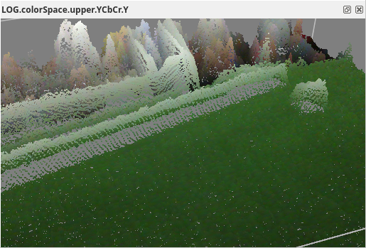
Color space views visualize image information in 3-D. They can be rotated by clicking into them with the left mouse button and dragging the mouse afterwards. There are two kinds of color space views:

• Image Color Channel: This view displays an image while using a certain color channel as height information (cf. the image above).
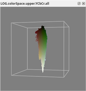
• Image Color Space: This view displays the distribution of all pixels of an image in a certain color space (HSI, RGB, or YCbCr). It can be displayed by selecting the entry all for a certain color space in the scene graph (cf. the image on the right).

The two kinds of views can be instantiated for the camera image (which is already done in most startup scripts) or any debug image. For instance, to add a set of views for the lower camera image under the name raw, the following command has to be executed:

Cognition¶

Field Views¶

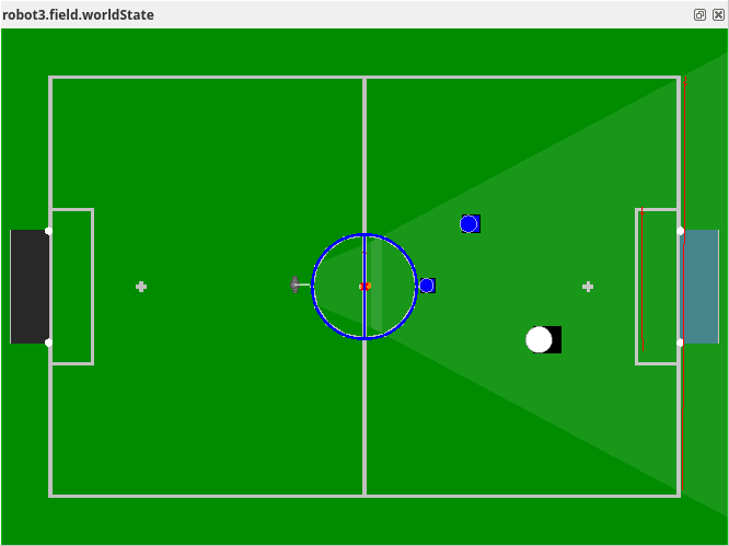
A field view displays information in the system of coordinates of the soccer field. The commands to create and manipulate it are defined similar to the ones for image views. For instance, the view worldState is defined as:

# field views
vf worldState
vfd worldState fieldLines
vfd worldState goalFrame
vfd worldState fieldPolygons
vfd worldState representation:RobotPose
# ...

# views relative to robot
vfd worldState cognition:RobotPose
vfd worldState representation:BallModel:endPosition
# ...

# back to global coordinates
vfd worldState cognition:Reset

Please note that some drawings are relative to the robot rather than relative to the field. Therefore, special drawings exist that change the system of coordinates for all drawings added afterwards, until the system of coordinates is changed again.

The field can be zoomed in or out by using the mouse wheel, touch gestures, or the page up/down buttons. It can also be dragged around with the left mouse button or by touch gestures. Double clicking the view resets it to its initial position and scale.

Behavior View ¶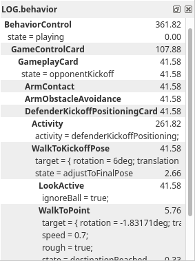

The behavior view shows all currently active cards and skills and the states they are in. Since the behavior consists of two passes, there are two instances of this view: once for the team behavior and once for the individual behavior. To be able to display both of them, the following debug requests must be sent (which are, however, already part of all startup scripts):

dr representation:ActivationGraph
dr representation:TeamActivationGraph

Motion¶

Sensor Data View¶

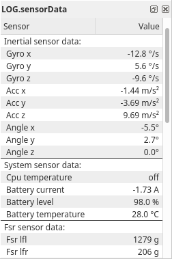The sensor data view displays all the sensor data taken by the robot that is not joint-related, e.g. accelerations, gyro measurements and foot pressure readings. To display this information, the following debug requests must be sent (which are, however, already part of all startup scripts):

dr representation:InertialSensorData
dr representation:SystemSensorData
dr representation:FsrSensorData
dr representation:KeyStates

Joint Data View ¶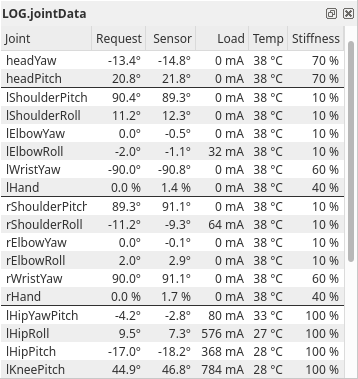

Similar to sensor data view, the joint data view displays all the joint data taken by the robot, e.g. requested and measured joint angles, temperatures, and loads. To display this information, the following debug requests must be sent (which are, however, already part of all startup scripts):

dr representation:JointRequest
dr representation:JointSensorData

Kick View¶

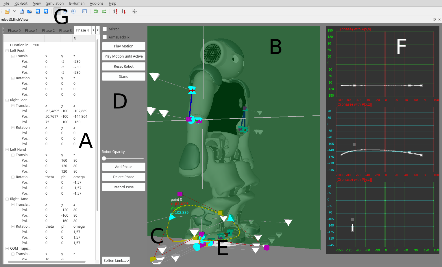
The idea of the kick view is to visualize and edit basic configurations of motions for the KickEngine described by Müller et al., 2011⁴. To do so, the central element of this view is a 3-D robot model. Regardless of whether the controller is connected to a simulated or a real robot, this model represents the current robot posture.

Since the KickEngine describes motions as a set of Bézier curves, the movement of the limbs can easily be visualized. Thereby the sets of curves of each limb are represented by combined cubic Bézier curves. Those curves are attached to the 3-D robot model with the robot center as origin. They are painted into the three-dimensional space. Each curve is defined by this equation:

To represent as many aspects as possible, the kick view has several sub views:

• 3-D View: In this view each combined curve of each limb is directly attached to the robot model and therefore painted into the 3-dimensional space. Since it is useful to observe the motion curves from different angles, the view angle can be rotated by clicking with the left mouse button into the free space and dragging it in one direction while holding the Shift key. In order to inspect more or less details of a motion, the view can also be zoomed in or out by using the mouse wheel or the page up/down buttons. The left/right arrow keys can translate the robot sidewards.

  A motion configuration is not only visualized by this view, it is also editable. The user can click on one of the visualized control points (cf. this image at E) and drag it to the desired position. In order to visualize the current dragging plane, a light green area (cf. this image at B) is displayed during the dragging process. This area displays the mapping between the screen and the model coordinates and can be adjusted by using the right mouse button and choosing the desired axis configuration.

  Another feature of this view is the ability to display unreachable parts of motion curves. Since a motion curve defines the movement of a single limb, an unreachable part is a set of points that cannot be traversed by the limb due to mechanic limitations. The unreachable parts will be clipped automatically and marked with orange color (cf. this image at C).

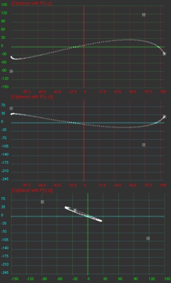• 1-D/2-D View: In some cases a movement only happens in the 2-dimensional or 1-dimensional space (e.g. raising a leg is a movement along the z-axis only). For that reason, more detailed sub views are required. Those views can be displayed as an overlay to the 3-D view by using the context menu, which opens by clicking with the right mouse button and choosing Display 1D Views or Display 2D Views. This only works within the left area where the control buttons are (cf. this image at D). By clicking with the right mouse button within the 3-D view, the context menu for choosing the drag plane appears. The second way to display a sub view is by clicking at the KickEdit entry in the title menu. This displays the same menu which appears as context menu.

  Because clarity is important, only a single curve of a single phase of a single limb can be displayed at the same time. If a curve should be displayed in the detailed views, it has to be activated. This can be done by clicking on one of the attached control points.

  The 2-D view (first image) is divided into three sub views. Each of these sub views represents only two dimensions of the activated curve. The curve displayed in the sub views is defined by this equation with \(P_i = {c_{x_i} \choose c_{y_i}}\), \(P_i = {c_{x_i} \choose c_{z_i}}\), or \(P_i = {c_{y_i} \choose c_{z_i}}\).

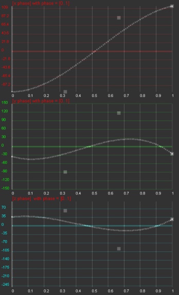  The 1-D sub views (second image) are basically structured as the 2-D sub views. The difference is that each single sub view displays the relation between one dimension of the activated curve and the time t. That means that in this equation \(P_i\) is defined as: \(P_i = c_{x_i}\), \(P_i = c_{y_i}\), or \(P_i = c_{z_i}\).

  As in the 3-D view, the user can edit a displayed curve directly in any sub view by drag and drop.

• Editor Sub View: The purpose of this view is to constitute the connection between the real structure of the configuration files and the graphical interface. For that reason, this view is responsible for all file operations (for example open, close, and save). It represents loaded data in a tabbed view, where each phase is represented in a tab and the common parameters in another one.

  By means of this view the user is able to change certain values directly without using drag and drop. Values directly changed will trigger repainting the 3-D view, and therefore, changes will be visualized immediately. This view also allows phases to be reordered by drag and drop, to add new phases, or to delete phases.

To save or load a motion the kick view has to be the active view. Appropriate buttons will appear in the tool bar (cf. this image at G).

Others¶

Module Views¶

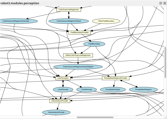
Since all the information about the current module configuration can be requested from the robot control program, it is possible to generate a visual representation automatically. The graphs, such as the one that is shown above, are generated by the program dot from the Graphviz package⁵. Modules are displayed as yellow rectangles and representations are shown as blue ellipses. Representations that are received from another thread are displayed in orange and have a dashed border. If they are missing completely due to a wrong module configuration or because they are alias representations, both label and border are displayed in red. The modules are separated into the categories that were specified as the second parameter of the macro MAKE_MODULE when they were defined. There are module views for the categories infrastructure, perception, communication, modeling, behaviorControl, sensing, and motionControl.

The module graph can be zoomed in or out by using the mouse wheel, touch gestures, or the page up/down buttons. It can also be dragged around with the left mouse button or by touch gestures.

Plot Views¶

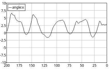
Plot views allow plotting data sent from the robot control program through the macro PLOT. They keep a history of the values sent, up to a defined size. Several plots can be displayed in the same plot view in different colors. A plot view is defined by giving it a name using the console command vp and by adding plots to the view using the command vpd (cf. this section). For instance, the view on the right was defined as:

vp orientationX 200 -10 10
vpd orientationX representation:InertialData:angle:x

Timing Views¶

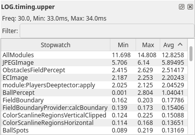The timing view displays statistics about all currently active stopwatches in a thread. It shows the minimum, maximum, and average runtime of each stopwatch in milliseconds as well as the average frequency of the thread. All statistics sum up the last 100 invocations of the stopwatch. Timing data is transferred to the PC using debug requests. By default the timing data is not sent to the PC. Execute the console command dr timing to activate sending timing data.

Data Views¶

SimRobot offers two console commands (get and set) to view or edit anything that the robot exposes using the MODIFY macro. While those commands are enough to occasionally change some variables, they can become quite annoying during heavy debugging sessions.

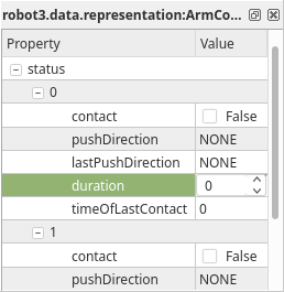
For this reason, the data view exists. It displays modifiable content using a property browser. Property browsers are well suited for displaying hierarchical data and should be well known from various editors such as Microsoft Visual Studio or Eclipse.

A new data view is constructed using the command vd in SimRobot. For example, vd representation:ArmContactModel will create a new view displaying the ArmContactModel. Data views can be found in the data category of the scene graph.

The data view automatically updates itself ten times per second. Higher update rates are possible, but result in a much higher CPU usage.

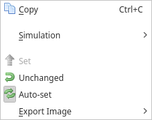To modify data, just click on the desired field and start editing. The view will stop updating itself as soon as you start editing a field. The editing process is finished either by pressing enter or by deselecting the field. By default, modifications will be sent to the robot immediately. This feature is called the auto-set mode. It can be turned off using the context menu. If the auto-set mode is disabled, data can be transmitted to the robot using the set item from the context menu.

Once the modifications are finished, the view will resume updating itself. However you may not notice this since modification continuously overwrites the data on the robot side, so the updated data are the same as entered in the data view. To stop overwriting the data, use the unchanged item from the context menu. As a result, the data will be unfrozen on the robot side and you should see the data changing again.

Log Player View¶

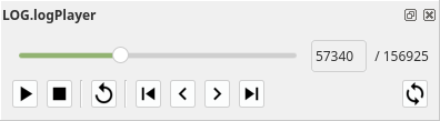
The log player allows to control the replay of log files using the following buttons:

Button	Function
	Start playback
	Stop playback
	Replay the current frame
	Go to the previous frame with an image
	Go to the previous frame
	Go to the next frame
	Go to the next frame with an image
	Run in a loop, i.e. continue at the beginning after the end is reached

In addition, the current frame can be directly entered as a number or selected using a slider.

Annotation View¶

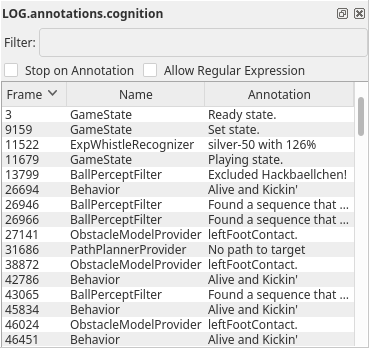The annotation view displays all annotations (cf. this section) contained in a log file. Double clicking an annotation will cause the log file to jump to the given frame number.

It is also possible to view annotations in real-time when using the simulated NAO or a direct debug connection to a real NAO. This has to be activated by using the following debug request:

dr annotation

Scene Description Files¶

The language of scene description files is an extended version of RoSiML¹. Scene files that use SimRobotCore2 have to end with .ros2, such as BH.ros2. In the following, the most important elements, which are necessary to add robots, dummies, and balls, are shortly described (based upon BH.ros2). For a more detailed documentation, see this chapter.

• <Include href="...">: First of all the descriptions of the NAO itself, a specific setup of NAOs, the ball and the field are included. The names of include files end with .rsi2.
• <Scene ...>: This element begins the instantiation section of the scene description. While everything outside the scene element, i.e. the files included above, only declares templates for objects, everything that follows is actually instantiated in the scene. The attributes of this element define some important properties of the scene, e.g. the controller library and the duration of each simulation step.
• <Compound name="teamColors">: This compound contains two appearances of which only the names matter. It defines the jersey colors of the two teams which the simulated GameController assumes. This is mainly important to make the jersey detection work in the simulation and does not have an effect on the actual appearance of the robots (see below).
• <Compound ref="robots"/>: This compound a macro that contains all active robots, i.e. robots for which will be controlled by the B-Human modules. However, each of them will require a lot of computation time. In the tag Body, the attribute ref specifies which NAO model should be used and name sets the robot name in the scene graph of the simulation. Legal robot names are "robot1" ... "robot12", where the first six robots are assumed to play in the first team (with player numbers 1...6) while the other six play in the second team (again with player numbers 1...6). The standard color of the NAO's jersey is set to black. To set it to red, use <Set name="NaoColor" value="red"> within the Body element.
• <Compound ref="extras"/>: This compound contains passive robots (or references a macro that does), i.e. robots that just stand around, but are not controlled by a program. Passive robots can be activated by moving their definition to the original compound robots and changing the referenced model from "NaoDummy" to "Nao".
• <Compound name="balls">: This compound contains an instance of the ball.
• <Compound ref="field"/>: This element instantiates the field from the included file as part of the scene.

Predefined Scenes¶

A lot of scene description files can be found in Config/Scenes. There are two types of scene description files: the ones required to simulate one or more robots, and the ones that connect to a real robot.

Simulating multiple robots is expensive. To overcome this and enable decent frame rates, some scenes come in special variants. In scenes ending with PerceptOracle, no camera images are rendered and percepts are provided by the simulator. However, models, for example the BallModel, still have to be calculated. This is different in the scenes with the suffix Fast, in which even the models are replaced with ground truth data from the simulator.

• BH[PerceptOracle|Fast]: A single robot with five dummies.
• OneTeam[PerceptOracle|Fast]: A team of five robots against dummies.
• Game[PerceptOracle|Fast]: A game five against five.
• KickViewScene[Remote]: For working on kicks (cf. this section).
• ReplayRobot: Replays a log file (cf. this section).
• RemoteRobot: Connects to a remote robot and displays images and data.

Console Commands¶

Console commands can either be directly typed into the console window or they can be executed from a script file. There are three different kinds of commands. The first kind will typically be used in a script file that is executed when the simulation is started. The second kind are global commands that change the state of the whole simulation. The third type is robot commands that affect currently selected robots only (see command robot to find out how to select robots).

Initialization Commands¶

• cl <location>: Changes the location that is used in the configuration file search path of simulated robots. This command is special, because it only has an effect if run directly from the script that is executed when a scene is loaded. This command and the following one are always executed before any other command in the script, because the location must be set before any robot code is executed, as otherwise configuration files would have already been loaded from the default path.
• cs <scenario> [team1|team2]: Changes the scenario that is used in the configuration file search path of simulated robots. As for the command cl, this command only has an effect if run directly from the script that is executed when a scene is loaded. This command and the previous one are always executed before any other command in the script, because the scenario must be set before any robot code is executed, as otherwise configuration files would have already been loaded from the default path. The optional second parameter can be used to set the scenario for only one of the two simulated teams.
• sc <name> <a.b.c.d>: Starts a remote connection to a real robot. The first parameter defines the name that will be used for the robot. The second parameter specifies the IP address of the robot. The command will add a new robot to the list of available robots using name, and it adds a set of views to the scene graph. When the simulation is reset or the simulator is exited, the connection will be terminated.
• sl <name> [<file>]: Replays a log file. The command will instantiate a complete set of threads and views. The threads will be fed with the contents of the log file. The first parameter of the command defines the name of the virtual robot. The name can be used in the robot command (see below), and all views of this particular virtual robot will be identified by this name in the tree view. The second parameter specifies the path to the log file. If the path is not an absolute path, Config/Logs is the base directory. .log is the default extension of log files. It will be automatically added if no extension is given. If no file is given at all, the previously started log file is used. When replaying a log file, the replay can be controlled by the Log Player (cf. this section) or the command log (see below). It is even possible to load a different log file during the replay.
• sml <directory>: Replays all log files in a directory and its subdirectories, each in its own robot instance.

Global Commands¶

• ar {<feature>} ( off | on ): Enables or disables the entire automatic referee or individual features. The features are placeBall, placePlayers, switchToSet, switchToPlaying, ballOut, freeKickComplete, clearBall, penalizeLeavingTheField, penalizeIllegalPosition, penalizeIllegalPositionInSet, and unpenalize.
• call <file> [<file>]: Executes a script file. A script file contains commands as specified here, one command per line. The default location for scripts is the Config/Scenes directory, their default extension is .con. If the optional script file is present, that one is executed instead.
• ci off | on | <fps>: Switches the calculation of images on or off. If an image frame rate is explicitly specified instead of on, that one is used instead of the default value of 60 Hz. The simulation of the robot's camera image costs a lot of time, especially if several robots are simulated. In some development situations, it is better to switch off all low level processing of the robots and to work with ground truth world states, i.e., world states that are directly delivered by the simulator. In such cases there is no need to waste processing power by calculating camera images. Therefore, it can be switched off. However, by default this option is switched on. Note that this command only has an effect on simulated robots.
• cls: Clears the console window.
• dt off | on | <fps>: Switches simulation dragging to real-time on or off. If a frame rate is explicitly specified instead of "on", that one is used instead of the default value of 83.3 Hz. Normally, the simulation tries not to run faster than real-time. Thereby, it also reduces the general computational load of the computer. However, in some situations it is desirable to execute the simulation as fast as possible. By default, this option is activated.
• echo <text>: Prints text into the console window. The command is useful in script files to print commands that can later be activated manually by pressing the Enter key in the printed line.
• gc initial | ready | set | playing | finished | goalByFirstTeam | goalBySecondTeam | kickOffFirstTeam | kickOffSecondTeam | manualPlacementFirstTeam | manualPlacementSecondTeam | goalKickForFirstTeam | goalKickOffForSecondTeam | pushingFreeKickForFirstTeam | pushingFreeKickForSecondTeam | cornerKickForFirstTeam | cornerKickForSecondTeam | kickInForFirstTeam | kickInForSecondTeam | penaltyKickForFirstTeam | penaltyKickForSecondTeam | gameNormal | gamePenaltyShootout | competitionPhasePlayoff | competitionPhaseRoundRobin | competitionTypeNormal: Sets the current state of the GameController.
• ( help | ? ) [<pattern>]: Displays a help text. If a pattern is specified, only those lines of the help are printed that contain the pattern.
• mvo <name> <x> <y> <z> [<rotx> <roty> <rotz>]: Moves the object with the given name to the given position and optionally rotates it.
• robot ? | all | <name> {<name>}: Selects a robot or a group of robots. The console commands described in the next section are only sent to selected robots. By default, only the robot that was created or connected last is selected. Using the robot command, this selection can be changed. Type robot ? to display a list of the names of available robots. A single simulated robot can also be selected by double-clicking it in the scene view. To select all robots, type robot all.
• st off | on: Switches the simulation of time on or off. Without the simulation of time, all calls to Time::getCurrentSystemTime() will return the real time of the PC. However if the simulator runs slower than real-time, the simulated robots will receive less sensor readings than the real ones. If the simulation of time is switched on, each step of the simulator will advance the time by 12 ms. Thus, the simulator simulates real-time, but it is running slower. By default this option is switched off.
• # <text>: Begins a comment line. Useful in script files.

Robot Commands¶

• bc [<red%> [<green%> [<blue%>]]]: Defines the background color for 3-D views. The color is specified in percentages of red, green, and blue intensities. All parameters are optional. Missing parameters will be interpreted as 0%.
• dr ? [<pattern>] | off | <key> ( off | on ): Sends a debug request. B-Human uses debug requests to switch debug responses (cf. this section) on or off at runtime. Type dr ? to get a list of all available debug requests. The resulting list can be shortened by specifying a search pattern after the question mark. Debug responses can be activated or deactivated. They are deactivated by default. Specifying just off as the only parameter returns to this default state. Several other commands also implicitly send debug requests, e.g. to activate the transmission of debug drawings.
• get ? [<pattern>] | <key> [?]: Shows debug data or shows its specification. This command allows displaying any information that is provided in the robot code via the MODIFY macro. If one of the strings that are used as first parameter of the MODIFY macro is used as parameter of this command (the modify key), the related data will be requested from the robot code and displayed. The output of the command is a valid set command (see below) that can be changed to modify data on the robot. A question mark directly after the command (with an optional filter pattern) will list all the modify keys that are available. A question mark after a modify key will display the structure of the associated data type rather than the data itself.
• jc hide | show | motion ( 1 | 2 ) <command> | ( press | release ) <button> <command>: Sets a joystick command. If the first parameter is press or release, the number following is interpreted as the number of a joystick button. Legal numbers are between 1 and 40. Any text after this first parameter is part of the second parameter. The <command> parameter can contain any legal script command that will be executed in every frame while the corresponding button is pressed. The prefixes press or release restrict the execution to the corresponding event. The commands associated with the 26 first buttons can also be executed by pressing Ctrl+Shift+A... Ctrl+Shift+Z on the keyboard. If the first parameter is motion, an analog joystick command is defined. There are two slots for such commands, number 1 and 2, e.g., to independently control the robot's walking direction and its head. The remaining text defines a command that is executed whenever the readings of the analog joystick change. Within this command, $1...$8 can be used as placeholders for up to eight joystick axes. The scaling of the values of these axes is defined by the command js (see below). If the first parameter is show, any command executed will also be printed in the console window. hide will switch this feature off again, and hide is also the default.
• jm <axis> <button> <button>: Maps two buttons on an axis. Pressing the first button emulates pushing the axis to its positive maximum speed. Pressing the second button results in the negative maximum speed. The command is useful when more axes are required to control a robot than the joystick used actually has.
• js <axis> <speed> <threshold> [<center>]: Sets the axis maximum speed and ignore threshold for command jc motion. axis is the number of the joystick axis to configure (1...8). speed defines the maximum value for that axis, i.e., the resulting range of values will be [-speed...speed]. The threshold defines a joystick measuring range around zero in which the joystick will still be recognized as centered, i.e., the output value will be 0. The threshold can be set between 0 and 1. An optional parameter allows for shifting the center itself, e.g. to compensate for bad calibration of a joystick.
• kick: Adds the KickEngine view to the scene graph.
• log ...: This command supports both recording and replaying log files. The latter is only possible if the current set of robot instances was created using the initialization command sl (cf. this section). This command has several sub-commands, i.e. the following commands are parameters of the log command, such as log start.
  • ? [<pattern>]: Prints statistics on the messages contained in the current log file. The optional pattern limits output to messages corresponding to the pattern.
  • mr [list]: Sets the provider of all representations from the log file to LogDataProvider. If list is specified the module request commands will be printed to the console instead.
  • start | stop: If replaying a log file, starts and stops the replay. Otherwise, the commands will start and stop the recording.
  • pause | forward [image] | backward [image] | repeat | goto <number> | time <minutes> <seconds> | fastForward | fastBackward: Controls replay of a log file. pause stops the replay without rewinding to the beginning, forward and backward advance a single step in the respective direction. With the optional parameter image, it is possible to skip all frames in between that do not contain images. repeat just resends the messages from the current frame. goto allows jumping to a certain frame in the log file. If the log file contains the representation GameInfo, the command time allows to jump to the first frame with a certain remaining game time. fastForward and fastBackward advance by 100 steps forward or backward.
  • cycle | once: Decides whether the log file is replayed only once or continuously repeated.
  • clear | ( keep | remove ) <message> {<message>} | keep ( ballPercept [seen | guessed] | ballSpots | circlePercept | lower | option <option> [<state>] | penaltyMarkPercept | upper ): clear removes all messages from the log file, while keep and remove only delete a selected subset based on the set of message IDs specified. keep also has a second form, in which a condition can be specified that is used to keep the frames (not just the messages) that meet the condition. The conditions are hardcoded in the implementation of the RobotConsole. They check, e.g., whether the image was recorded from a specific camera, a certain object was detected or the behavior was in a specific state in a frame.
  • ( load | save [split <parts>] ) <file>: These commands load or save the log file stored in memory from or to a file, respectively. If the filename is not a absolute path, it is relative to Config/Logs. Otherwise, the full path is used. .log is the default extension of log files. It will be automatically added if no extension is given. When saving a log file, it can be split into a specified number of parts with an equal number of messages.
  • trim ( until <end frame> | from <start frame> | between <start frame> <end frame> ): Keeps only the given section of the log and saves the log file afterwards.
  • saveAudio [<file>]: Saves the audio data from the current log file to a .wav file. If no filename is given, the file is created at the log file's location with the .wav extension. If the specified filename is not an absolute path, it is relative to Config/Sounds.
  • saveImages [raw] [onlyPlaying] [<takeEachNth>] [<dir>]: Saves images from the current log file as PNG files to a directory. If raw is specified, images are left in their YUV format, otherwise they are converted to RGB. onlyPlaying only selects images that were taken while the robot was in the playing state, unpenalized and upright. Images can be skipped using the parameter takeEachNth. If no target directory is given, the images are put in a new directory next to the log file. If the specified directory is not an absolute path, it is relative to Config/Images.
  • ( saveInertialSensorData | saveJointAngleData ) [<file>]: Saves sensor data from the current log file to a .csv file. If no filename is given, the file is created at the log file's location with the .csv extension.
  • saveLabeledBallSpots [<file>]: Saves image patches around ball spots from the current log file, including a .csv file with label information. For this, the representation LabelImage must be present in the log file, which has to be patched in by an external annotation tool. The image patches are stored in a new directory at the log file's location.
  • saveTiming [<file>]: Saves timing data from all stopwatches for each frame from the current log file to a .csv file. If no filename is given, the file is created at the log file's location with the .csv extension.
  • full | jpeg: Decides whether uncompressed images received from the robot will also be written to the log file as full images, or JPEG-compressed on the recording PC before. When the robot is connected by cable, sending uncompressed images is usually a lot faster than compressing them on the robot. By executing log jpeg, they can still be saved in JPEG format, saving memory space during recording as well as disk space later. Note that running image processing routines on JPEG images does not always give realistic results, because JPEG is not a lossless compression method, and it is optimized for human viewers, not for machine vision.
• msg off | on | log <file> | disable | enable: Switches the output of text messages on or off, or redirects them to a text file. All threads can send text messages via their message queues to the console window. As this can disturb entering text into the console window, printing can be switched off. However, by default text messages are printed. In addition, text messages can be stored in a log file, even if their output is switched off. The file name has to be specified after msg log. If the file already exists, it will be replaced. If no path is given, Config/Logs is used as default. Otherwise, the full path is used. .txt is the default extension of text log files. It will be automatically added if no extension is given. enable and disable can switch between handling messages from the robot at all, which is enabled by default.
• mr ? [<pattern>] | modules [<pattern>] | save | <representation> ( ? [<pattern>] | ( <module> | off ) [<thread>] | default ): Sends a module request. This command allows selecting the module that provides a certain representation in a certain thread. If the representation is currently provided in exactly one thread, the thread argument can be omitted. If a representation should not be provided anymore, it can be switched off. Deactivating the provision of a representation is usually only possible if no other module requires that representation. Otherwise, an error message is printed and the robot is still using its previous module configuration. Sometimes, it is desirable to be able to deactivate the provision of a representation without the requirement to deactivate the provision of all other representations that depend on it. In that case, the provider of the representation can be set to default. Thus no module updates the representation and it simply keeps its previous state. A question mark after the command lists all representations. A question mark after a representation lists all modules that provide this representation. The parameter modules lists all modules with their requirements and provisions. All three listings can be filtered by an optional pattern. save saves the current module configuration to the file threads.cfg which it was originally loaded from. Note that this usually has not the desired effect, because the module configuration has already been changed by the start script to be compatible with the simulator. Therefore, it will not work anymore on a real robot. The only configuration in which the command makes sense is when communicating with a remote robot.
• mv <x> <y> <z> [<rotx> <roty> <rotz>]: Moves the selected simulated robot to the given position and rotates it if a rotation is specified. x, y, and z have to be specified in mm, the rotations have to be specified in degrees. Note that the origin of the NAO is about 330 mm above the ground, so z should be 330.
• mvb <x> <y> <z>: Moves the ball to the given position. x, y, and z have to be specified in mm. Note that the radius of the ball is 50 mm above the ground, so z should be at least 50.
• poll: Polls for all available debug requests and debug drawings. Debug requests and debug drawings are dynamically defined in the robot control program. Before console commands that use them can be executed, the simulator must first determine which identifiers exist in the code that currently runs. Although the acquisition of this information is usually done automatically, e.g. after the module configuration was changed, there are some situations in which a manual execution of the command poll is required. For instance if debug responses or debug drawings are defined inside another debug response, executing poll is necessary to recognize the new identifiers after the outer debug response has been activated.
• pr none | illegalBallContact | playerPushing | illegalMotionInSet | inactivePlayer | illegalPosition | leavingTheField | requestForPickup | localGameStuck | illegalPositionInSet | substitute | manual | unstiff | active | calibration: Penalizes a simulated robot with the given penalty, unpenalizes it when used with none, or set the robot's state. If the automatic referee is turned on, the necessary placement is done automatically: When penalized, the simulated robot will be moved to the sideline, looking away from the field. When unpenalized, it will be turned, facing the field again, and moved to the sideline that is further away from the ball.
• save ? [<pattern>] | <key> [<path>]: Save debug data to a configuration file. The keys supported can be queried using the question mark. An additional pattern filters the output. If no path is specified, the name of the configuration file is looked up from a table, and its first occurrence in the search path is overwritten. Otherwise, the path is used. If it is relative, it is appended to the directory Config.
• set ? [<pattern>] | <key> ( ? | unchanged | <data>): Changes debug data or shows its specification. This command allows changing any information that is provided in the robot code via the MODIFY macro. If one of the strings that are used as first parameter of the MODIFY macro is used as parameter of this command (the modify key), the related data in the robot code will be replaced by the data structure specified as second parameter. It is best to first create a valid set command using the get command (see above). Afterwards that command can be changed before it is executed. If the second parameter is the key word unchanged, the related MODIFY statement in the code does not overwrite the data anymore, i.e. it is deactivated again. A question mark directly after the command (with an optional filter pattern) will list all the modify keys that are available. A question mark after a modify key will display the structure of the associated data type rather than the data itself.
• si reset [<number>] | ( upper | lower ) [number] [grayscale] [<file>]: Saves the raw image of a robot. The image will be saved in the format derived from the file extension in color, unless the grayscale option is specified. If no path is specified, Config/raw_image.bmp will be used as default. If number is specified, a number is appended to the filename that is increased each time the command is executed. The option reset resets the counter to a specified value or 0 if none is specified.
• v3 ? [<pattern>] | <image> [jpeg] <[thread>] [<name>]: Adds a set of 3-D color space views for a certain image (cf. this section). The image can either be the camera image (simply specify image) or a debug image. The camera image can also be JPEG-compressed by using the jpeg option. By default, the debug image is taken from the Lower thread. However, the thread parameter can switch to the image from another thread. The last parameter is the name that will be given to the set of views. If the name is not given, it will be the same as the name of the image plus the name of the thread from which the image is taken. A question mark followed by an optional filter pattern will list all available images.
• vd <debug data> ( on | off ): Adds a data view (cf. this section) for debug data that is provided in the robot code via the MODIFY macro. Data views can be found in the data category of the scene graph. They provide the same functionality as the get and set commands (see above). However they are much more comfortable to use.
• vf <name>: Adds a field view (cf. this section). A field view is the means for displaying debug drawings in field coordinates. The parameter defines the name of the view.
• vfd ? [<pattern>] | off | ( all | <name> ) ( ? [<pattern>] | <drawing> ( on | off ) ): (De)activates a debug drawing in a field view. The first parameter is the name of a field view that has been created using the command vf (see above) or all to add the drawing to all field views. The second parameter is the name of a drawing that is defined in the robot control program. Such a drawing is activated if the third parameter is on or is missing. It is deactivated if the third parameter is off. The drawings will be drawn in the sequence they are added, from back to front. Adding a drawing a second time will move it to the front unless the drawing is an origin drawing (those can be "drawn" multiple times). A question mark directly after the command will list all available field views. A question after a valid field view will list all available field drawings. Both question marks have an optional filter pattern that reduces the number of answers. vfd off will turn off all debug drawings except for the background in all field views.
• vi ? [<pattern>] | <image> [jpeg] [<thread>] [<name>] [ gain <value>] [ddScale <value>]: Adds an image view (cf. this section). An image view is the means for displaying debug drawings in image coordinates. The image can either be the camera image (simply specify image), a debug image, or no image at all (none). The camera image can also be JPEG-compressed by using the jpeg option. By default, the debug image is taken from the Lower thread. However, the thread parameter can switch to the image from another thread. The next parameter is the name of the view that is needed when adding drawings to it. If the name is not given, it will be the same as the name of the image and the name of the thread from which the image is taken. With the argument of the gain parameter the image gain can be adjusted, if no gain is specified the default value will be 1.0. The argument of ddScale can set a custom scaling of debug drawings in the view, which is 1.0 by default. A question mark followed by an optional filter pattern will list all available images.
• vic ? [<pattern>] | ( all | <name> ) [alt | noalt] [ctrl | noctrl] [shift | noshift] <command>: Sets a command to be executed when clicking on an image view. The first parameter is the name of an image view that has been created using the command vi (see above) or all to set the command for all image views. Then, for the modifier keys Alt, Control and Shift, it can be selected whether they either must or must not be pressed while clicking for the command to be executed. Modifiers that are not mentioned at all are ignored. Everything after the modifier specification is the command that will be executed on clicking the image view. In the command, the placeholders $1...$3 can be used to insert the x-coordinate, y-coordinate and the lower case thread identifier to which the image view belongs, respectively. A question mark directly after the command will list all available image views.
• vid ? [<pattern>] | off | ( all | <name> ) ( ? [<pattern>] | <drawing> ( on | off ) ): (De)activates a debug drawing in an image view. The first parameter is the name of an image view that has been created using the command vi (see above) or all to add the drawing to all image views. The second parameter is the name of a drawing that is defined in the robot control program. Such a drawing is activated if the third parameter is on or is missing. It is deactivated if the third parameter is off. The drawings will be drawn in the sequence they are added, from back to front. Adding a drawing a second time will move it to the front. A question mark directly after the command will list all available image views. A question mark after a valid image view will list all available image drawings. Both question marks have an optional filter pattern that reduces the number of answers. vid off will turn off all debug drawings in all image views.
• vp <name> <numOfValues> <minValue> <maxValue> [<yUnit> [<xUnit> [<xScale>]]]: Adds a plot view (cf. this section). A plot view is the means for plotting data that was defined by the macro PLOT in the robot control program. The first parameter defines the name of the view. The second parameter is the number of entries in the plot, i.e. the size of the x axis. The plot view stores the last numOfValues data points sent for each plot and displays them. minValue and maxValue define the range of the y axis. The optional parameters can improve the appearance of the plots by adding labels to both axes and by scaling the time-axis. The axis label drawing can be toggled by using the context menu of the plot view.
• vpd ? [<pattern>] | <name> ( ? [<pattern>] | <drawing> ( ? [<pattern>] | <color> [<description>] | off ) ): Plots data in a certain color in a plot view. The first parameter is the name of a plot view that has been created using the command vp (see above). The second parameter is the name of plot data that is defined in the robot control program. The third parameter defines the color for the plot. white, black, red, green, blue, yellow, cyan, magenta, orange, violet, gray, brown, and six-digit hexadecimal RGB color codes are supported. An optional fourth parameter can set a custom description of the plot data. The plot is deactivated when the third parameter is off. The plots will be drawn in the sequence they were added, from back to front. Adding a plot a second time will move it to the front. A question mark directly after the command will list all available plot views. A question after a valid plot view will list all available plot data. A question mark after a valid plot view and a valid plot data identifier will list the available colors. All question marks have an optional filter pattern that reduces the number of answers.

Input Dialogs¶

Input dialogs may be used as placeholders in scripting-files to request input from the user. The dialogs will be opened before their respective script-lines are executed and the user selected value handled as usual script, e.g. a command or parameter. In the following list, the outer curly braces are literals.

• ${<label>}: This expression opens a plain text input dialog.
• ${<label>,<relativePath>}: This expression opens a file selection dialog at the relative path. The path may also specify legal file names via the asterisk-character (*). This is used, e.g., in the file Config/Scenes/Include/replayDialog.con: ${Log File:,../../Logs/*.log}.
• ${<label>,,<relativePath>}: This expression opens a directory selection dialog at the relative path.
• ${<label>,<value-1>,<value-2>{,<value-n>}}: This expression opens a drop-down list with the respective name and value options. This is used, e.g., to open an IP address dialog in the file Config/Scenes/Include/connectDialog.con: ${IP address:,10.0.1.1,192.168.1.1}.